When you think of a Classpad, the first thing that probably comes to mind is a bulkier calculator. And you’d be right. It’s thicker, heavier, and has one massive screen. But like most celebrity gym-goers, the Classpad’s bulk is not natural - it’s truly a calculator on steroids.

Classpads are essentially mini computers, complete with their own file systems, user programmability, and processing power that humbles scientific calculators. However, its most impressive feature - at least to us students - is its mathematical functionality. Having Classpad proficiency gives you a significant advantage when facing calc-assumed tests. So, it’s always best to get to know your Classpad’s functions and be aware of what processes it can speed up for you.

With Classpads costing as much as Ed Sheeran tickets, you’ll definitely want the full mathematical tour. In this article, I’ll be going over how you can optimize your Classpad use, including the essential functions you should know about and little tricks that can speed things up. That way, you’ll get the full $300 worth in your tests and exams.

Please note that certain sections or discussions of functions may only be relevant to topics you haven’t covered yet. Nevertheless, I recommend that you read along to those sections as you may still obtain insights relevant to Classpad usage in the topics you have learned.

Main

Let’s start with the basics. The Main tab is the tab where you’ll be doing most of your calculations during a test. Therefore, it’s essential to know what all the buttons do and which ones will be relevant to you.

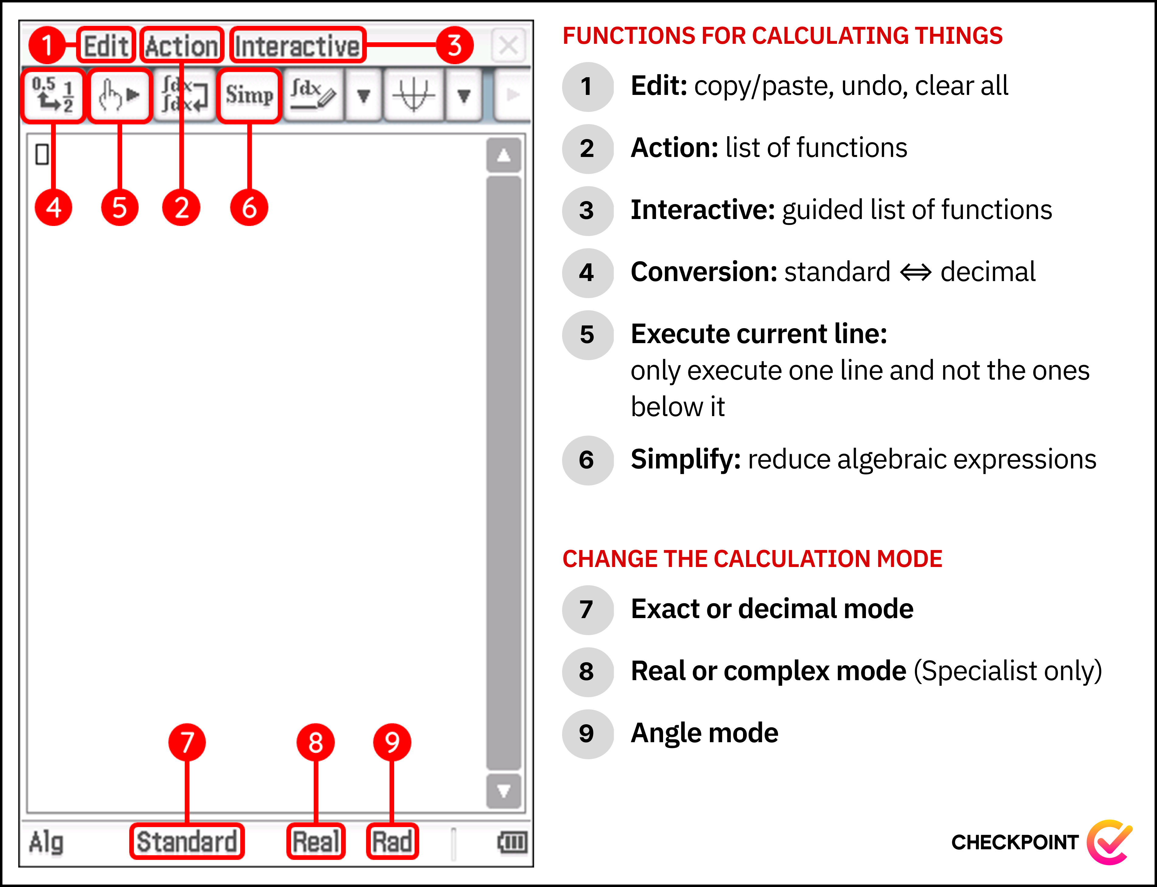
1. Edit - basic editing tools like copy/paste/clear

This menu is often overlooked, but is incredibly useful to us. The most important action the drop-down menu gives access to is Clear All, which many of you may already be familiar with. Clear All erases all calculations done on the Main tab, leaving you with a blank page. This is best done just before a test, as it removes any distracting calculations and reduces the overall vertical height of the page, making it easier to find specific calculations when checking your answers. Undo/Redo is another useful action from this menu to keep in mind, especially for those times when you spend ages typing out a massive equation only for it to be accidentally erased by pressing the clear button. Other useful functionalities include copying and pasting, which can also be done through the keyboard.

2. Action - a collection of useful tools

This menu provides us with a large selection of functions that we may use for our calculations (we cover these functions later). Upon selecting a function, it will be typed directly onto the main page and will require you to type in the function’s arguments (the input values of the function) in order separated by commas. For example, in Year 12 Methods, you’ll be using a function called binomialPDF. From the Action menu, we would go Distribution/Inv. Dist > Discrete > binomialPDF which would result in this:

[eyes] Notice that the function name is simply typed out, and we must type in the arguments in order ourselves.

3. Interactive - action, but easier to use

You’ll notice that this menu is exactly the same as Action, however when you select a function, it will take you to a new menu that shows input fields and labels for each argument. With our binomialPDF example, it would take us to a menu like this:

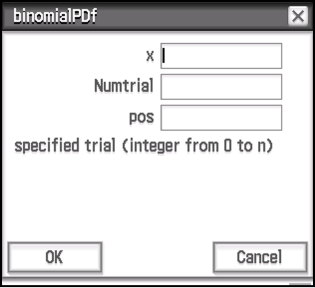
Here, we can see that the three required arguments are displayed, and selecting an input field will show a brief description of what that input field represents. In this example, the x input field is selected, and the description indicates that it represents the specified trial. Once all the parameters are provided and the OK button is pressed, the Classpad will automatically type out the function into the main section with the arguments provided in each input field.

So, why are there both Action and Interactive options? While Interactive is more user-friendly, it is slightly slower than typing out the arguments yourself in a single line on the main section. Additionally, since we can only hold one value on our clipboard, and the Interactive window blocks the view of our calculations on the main section, it becomes challenging when multiple arguments need to come from values in earlier calculations. My advice is to use Action if you’re comfortable with the argument order of a function, and otherwise use Interactive.

4. Standard to Decimal

This button allows you to convert an answer between exact and decimal representations. To use it, simply place your cursor on a calculation expression or an answer and press the button. Your Classpad will then have to re-execute the calculation to switch the answer’s representation.

5. Execute Current Line - when we want to make changes quickly

Typically, when we press EXE to execute a calculation, our Classpad will execute the calculation on the current line of our cursor and any lines below it (unless our cursor is already on the lowest line). This can be very useful, especially if we have used the ans button in successive calculations to use the answer from the previous calculation as all calculations will be updated accordingly. However, there may be times when we only want the current line of our cursor to be executed, because we don’t want our Classpad to waste time on lower calculations. In this case, we can use this button instead of EXE.

6. Simplify - does the grade 8 algebra for you

This button is as simple as the name, it tries to simplify the answer of the selected calculation. Simplify is actually a function but pressing the button will automatically place everything on the current line inside the Simplify function. Alternatively, pressing Simplifyon a blank line will simplify the previous answer.

7. Standard to Decimal, again

This is very similar to number 5 except instead of switching the representations (decimal or exact) of an answer on a line, this changes the default representation for all answers calculated from now on. This is why this button doesn’t change anything on the main page when it’s clicked as it is storing the selected setting for future calculations.

8. Real and Complex

This changes the set of numbers that the Classpad works with between just real numbers and complex numbers (which includes real numbers). Your Classpad will take longer to do certain calculations in Complex mode as it also searches for complex answers. This means that this setting should always be set to Real unless we are specifically doing a complex numbers calculation in Year 12 Specialist.

9. Angle representation and type

This changes how angles are represented in answers, and more importantly how angles are interpreted in calculations. Throughout Methods and Specialist, you’ll be switching between radians and degrees a lot (the third representation - gradians - won’t ever be used). This means that care must be taken when executing a calculation that involves an angle as we have to make sure the value of the angle we typed will be interpreted using the correct angle system.

Common functions

Action and Interactive

In the previous section, I gave an overview of the Action/Interactive menus and how they can help you execute calculations more efficiently than typing out all the working ourselves. Therefore, it’s important to have a good understanding of the available functions in these menus, especially the ones that are relevant to our course. The table below provides information on the functions that you should be aware of for each course.

Generally useful functions

Course	Function	Path	Arguments	Usage
General	expand	Transformation > expand	Any expression	Expands an expression.
General	factor	Transformation > factor	Any expression	Factorises an expression.
Yr 11/12 Methods	tanLine	Calculation > line > tanLine	Any expression, target variable, target value	Determines the equation for the line tangent to the function given in the expression when the target variable = target value. Although we would be using this function with single-variable expressions (likely with the target variable always being $x$), this function can be used with multi-variable expressions which is why there is an argument for target variable.
Yr 11/12 Methods	normal	Calculation > line > normal	Any expression, target variable, target value	Determines the equation for the line perpendicular to the function given in the expression when the target variable = target value. Same deal with the target variable argument as mentioned in the tanLine function.
Yr 11/12 Methods	fMin	Calculation > fMin/fMax > fMin	Any expression, target variable, lower bound, upper bound	Determines the absolute minimum of the function specified in the expression between the given bounds for the target variable and the value(s) of the target variable required for this to occur. The term absolute minimum is used as this is different from a local minimum. Unlike a local minimum, this function may output the value of the function at the bounds if it is smaller than any of the minimum turning points. E.g. the absolute minimum of $x^2$ is $-\infty$. Same deal with the target variable argument as mentioned in the tanLine function.
Yr 11/12 Methods	fMax	Calculation > fMin/fMax > fMax	Any expression, target variable, lower bound, upper bound	Determines the absolute maximum of the function specified in the expression between the given bounds for the target variable and the value(s) of the target variable required for this to occur. As explained in the fMin description for minimums, the absolute maximum is different to local maximums. Same deal with the target variable argument as mentioned in the tanLine function.
Yr 12 Spec	compToPol	Complex > compToPol	Any complex number	Converts a complex number to polar form. If it is already in polar form, this doesn’t change anything. Note that Classpads displays polar form in Euler form. In Euler form, the coefficient of the e is the magnitude and the coefficient of i in the exponent is the argument.
Yr 12 Spec	compToRect	Complex > compToRect	Any complex number	Converts a complex number to rectangular form ($a + bi$). If it is already in rectangular form, this doesn’t change anything. As mentioned in compToPol, the Classpad uses Euler notation for polar form complex numbers so you will have to write polar form inputs in that format.
Yr 11/12 Spec	angle	Vector > angle	Any vector, any vector	Determines the angle between the two given vectors
Yr 11/12 Spec	norm	Vector > norm	Any vector	Determines the magnitude of the given vector
Yr 12 Spec	crossP	Vector > crossP	Any vector, any vector	Determines the cross product of the given two vectors
Yr 11/12 Spec	dotP	Vector > dotP	Any vector, any vector	Determines the dot product of the given two vectors
Yr 12 Methods	normCDF	Distribution/Inv. Dist > Continuous > normCDF	Lower bound, upper bound, standard deviation, mean	Determines the probability of a normally distributed continuous random variable being between two values given the random variable’s mean and standard deviation
Yr 12 Methods	binomialPDF	Distribution/Inv. Dist > Discrete > binomialPDF	Target value, number of trials, probability of event	Determines the probability of a binomially distributed discrete random variable being a particular value given the number of trials in this binomial event and the probability of a success
Yr 12 Methods	binomialCDF	Distribution/Inv. Dist > Discrete > binomialCDF	Lower bound, upper bound, number of trials, probability of event	Determines the probability of a binomially distributed discrete random variable being between two values (inclusive) given the number of trials in this binomial event and the probability of a success
Yr 12 Methods	invNormCDF	Distribution/Inv. Dist > Inverse > invNormCDF	Tail direction, probability of region, standard deviation, mean	Determines the value such that the probability of a normally distributed continuous random variable with given mean and standard deviation satisfying a certain inequality is true depending on the mode chosen for tail direction. Tail direction - Left $P(X < \text{value}) = \text{probability}$ Tail direction - Right $P(X > \text{value}) = \text{probability}$ Tail direction - Center $P(\text{value} < X < \text{mean} \times 2 - \text{value}) = \text{probability}$

A quick note to make is that some of these functions may solve a question in less steps than the marking key intends, and hence run the risk of you losing marks for not showing all working.

For example, a typical “find the tangent to the function $f(x)$ at $x = a$” question will have marks given for

1. Finding the derivative at the correct $x$ value
2. Inserting this as the gradient in the $y = mx + c$ formula
3. Substituting coordinates to solve for $c$

Using the tanLine function to do this all in one go is unlikely to receive full marks.

A good rule of thumb is that questions that are worth 3 marks or more will require more than a single line of working with a single answer from your Classpad. However, this does not mean that these functions are irrelevant. We can still use these functions to quickly and reliably check our answers once we’ve written the full working.

The solve(⋅) Function

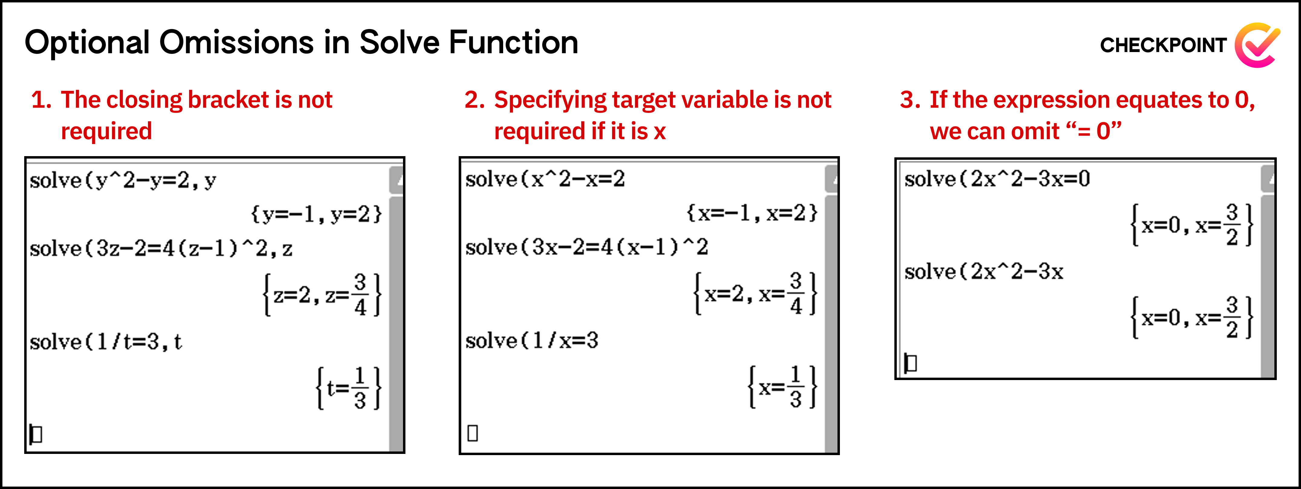
The solve() function is an extremely useful function found in that you’ll extensively use in almost all chapters of Methods and Specialist. The basic functionality of solve is solving for the exact value or values of a single variable. In these cases, we simply write solve(, followed by the mathematical equation, and lastly the variable you’re solving for after a comma (e.g. solve(x + 4x^2 = 3, x)). Note how we do not need to rearrange the expression to isolate $x$ - the Classpad will do that for us when it solves the equation!

Additionally, our Classpad does allow us to skip some of the details for certain situations.

1. We don’t need to write the closing bracket as your Classpad will assume you meant to write one (this actually applies to all functions)
2. We don’t need to specify the target variable if the target variable is $x$ as your Classpad will default to $x$
3. We don’t need to write the equality if the expression equals 0 as your Classpad defaults to the expression being equated to 0

Simultaneous equations

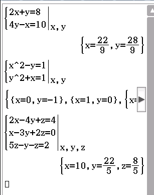
As an extension of solve(), the Classpad also provides functionality for solving simultaneous equations. To start typing a simultaneous equation, open the Math1 keyboard and press the button shown below

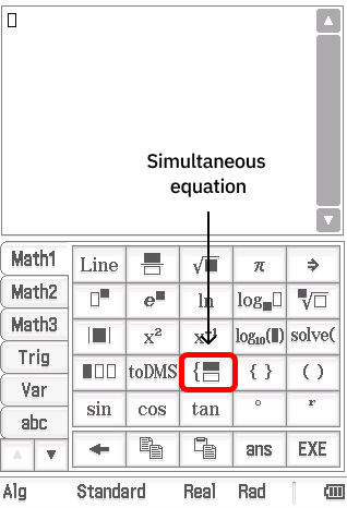
Next, simply type out each equation in your simultaneous system on to a separate line. By default this function will produce two lines. To add more, we can press the simultaneous equation button again while our cursor is inside the simultaneous system on our screen. Before pressing execute, we need to tell our Classpad which variables we are solving for, which can be done by typing them in the input field to the right of the vertical line and separating each variable by a comma.

Advanced keyboard

Fortunately, for most of our needs, we can easily access the required functions from Action/Interactive or the 3 math keyboards (Math1, Math2, Math3). The only exceptions are the functions required for combinatorics in Year 11 Specialist and Year 11/12 Methods courses. However, these can be easily accessed through the Advance keyboard located on the second page of keyboards. To access the Advance keyboard, simply press the down arrow located below the abc keyboard. The functions related to combinatorics that we need to be aware of are:

Course	Function	Path	Arguments	Usage
Yr 11 Spec and Yr 11 Methods	!	Advance > !	(This one isn’t really a function, we just need to write the number we want to apply the factorial operation to before the symbol)	Applies the factorial operation to the number before the symbol
Yr 11 Spec and Yr 11 Methods	nPr	Advance > nPr	Number of objects, Number of positions	Applies the permutations formula with the given parameters for $n$ and $r$
Yr 11 Spec and Yr 11/12 Methods	nCr	Advance > nCr	Number of objects, Number of selections	Applies the combinations formula with the given parameters for $n$ and $r$

Tabs other than main

So far we’ve only focused on the main tab (and for good reason, but we’ll get to that later). Although there are many others, there are only a handful that we’ll need to use for our test questions. These are Graph&Table, Statistics, eActivity and DiffEqGraph.

Graph & Table

Graph&Table is mainly used for visualising the graphs of functions. We simply type in the equation of the graph, tick the corresponding line and hit the graphing button (top left). This will cause all ticked equations to be graphed on the same set of axis. By default, your Classpad’s Graph&Table function type is set to explicit functions (functions that can be represented in the form $y = f(x)$) but this can be changed using the Type menu at the top. For example in Yr 12 Spec you’ll be graphing parametric equations and so will need to set the function type to ParamType.

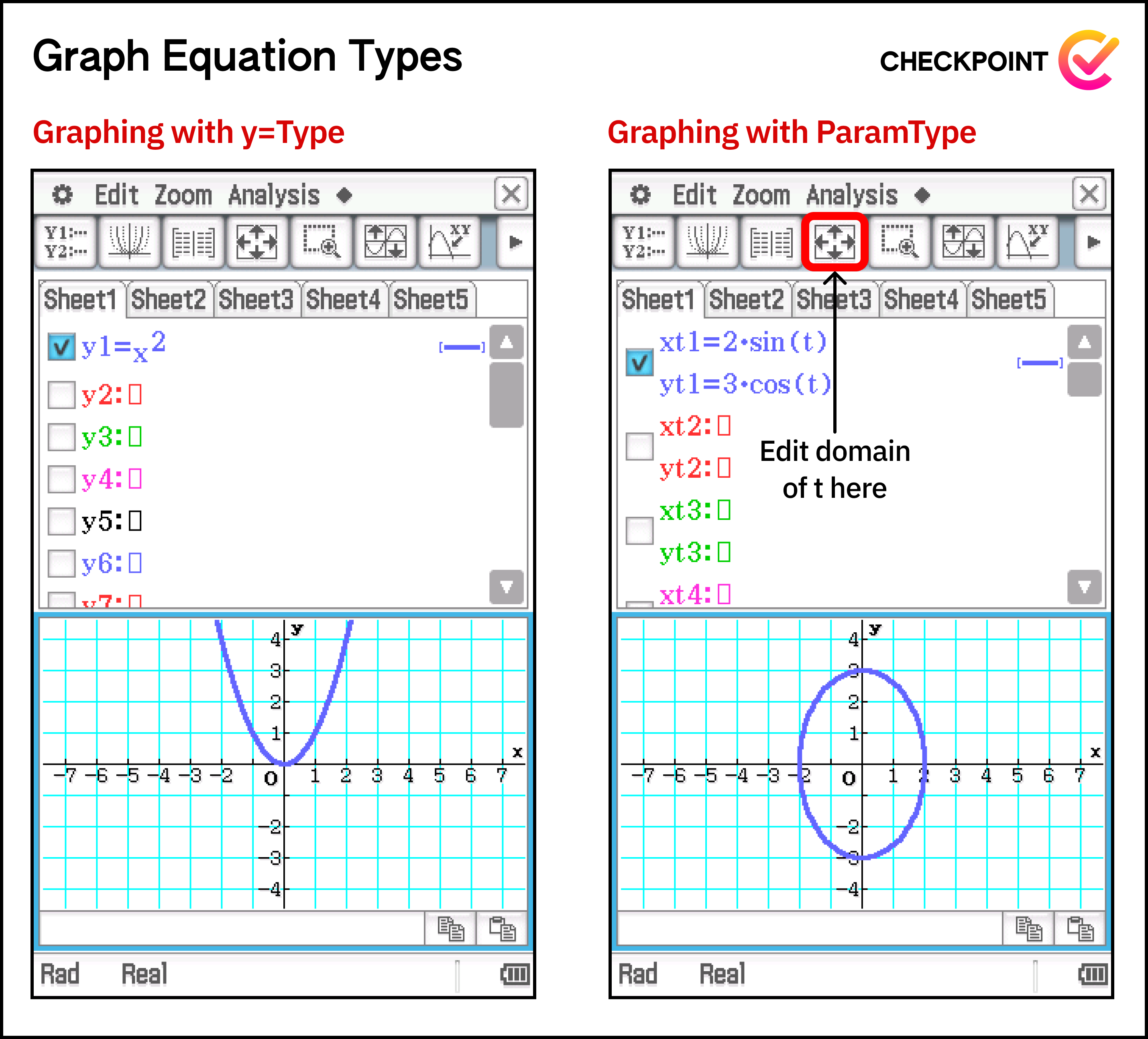
[warning] Note: when using ParamType, you may have to edit the domain of $t$ used for graphing. This can be done through the menu accessed by clicking the button with the 4 arrows

Graph&Table can also be used to find information about functions such as intercepts, turning points and intersections with other functions. These can be accessed through Analysis > G-Solve. If there are multiple turning points or intersections, we can use the arrow keys to move between them.

It is also a good idea to familiarise yourself with the different zoom options. The ones I commonly use are:

• Auto - your Classpad will try to decide which level of zoom is best
• Initialise - takes you to the Classpad’s default zoom ($x$-axis from $-7$ to $7$, $y$-axis from $-4$ to $4$)
• Box - allows you to draw a box that will be the border of the zoom (useful for when the Auto zoom shows too much of the graph)

Statistics

Statistics is almost only relevant for Yr 12 Methods as is used to find information about discrete random variables such as their mean, variance and standard deviation. To make use of this tab for Yr 12 Methods, we want to write the $x$-values in one column and the corresponding probabilities in another. These columns can be arbitrarily chosen, but to maintain consistency let’s make list1 contain the x-values and list2 contain their probabilities. After writing these values, we can find their statistics through Calc > One-Variable and setting XList to list and Freq to list2.

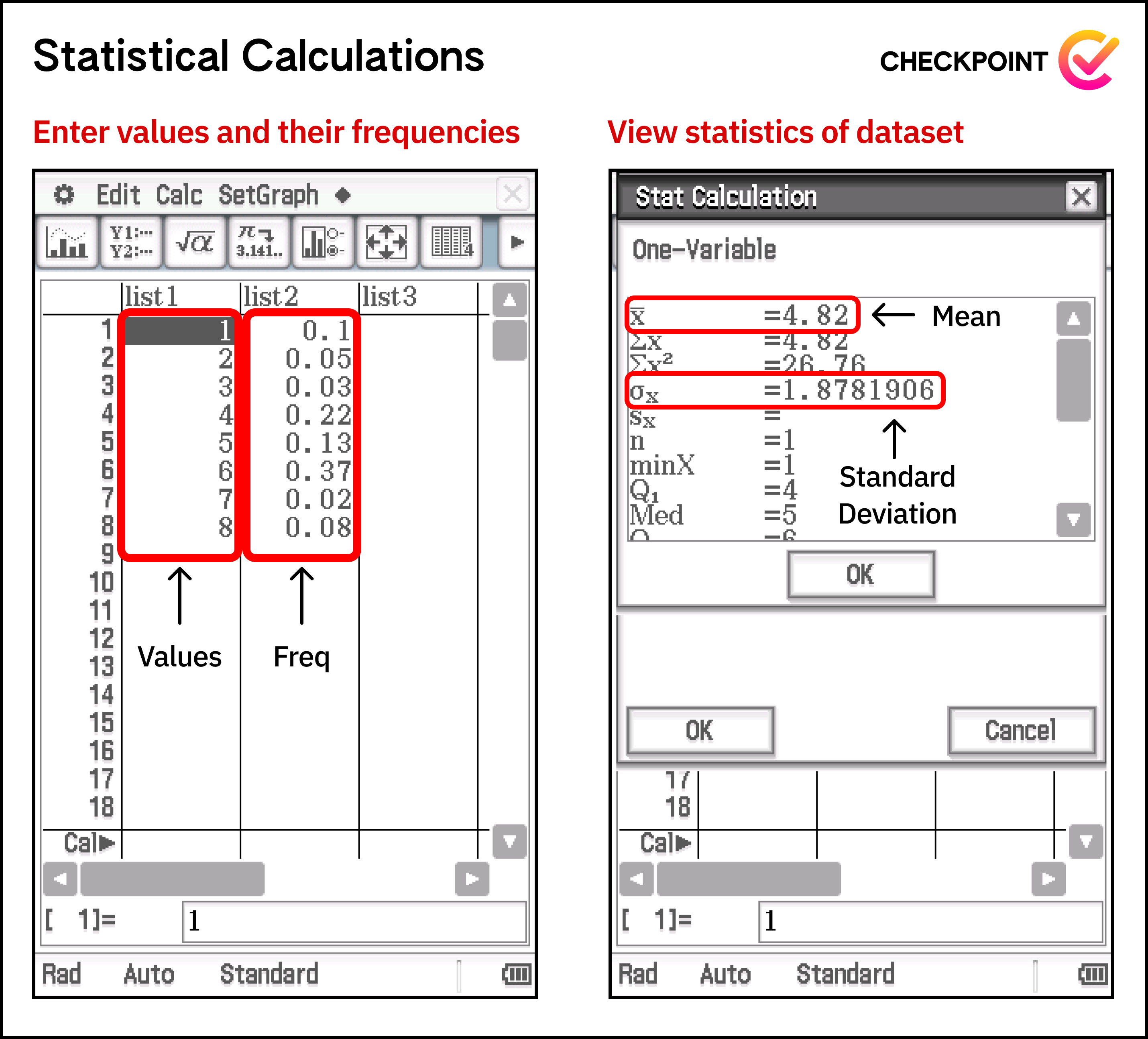
[eyes] Notice that the Stat Calculation represents mean with the symbol $\bar{x}$ and the standard deviation with symbol $\sigma_x$. Although the variance isn’t given, we can simply square the standard deviation.

One downside to the Statistics tab is that it does not allow us to copy values from the Stat calculation, making it quite annoying when we need to use the mean or standard deviation for further calculations. Therefore, sometimes it may just be better to perform the calculation for mean, variance or standard deviation in main using their formulas.

Differential Equations Graph

DiffEqGraphis only relevant to Yr 12 Spec and is used to visualise slope fields. To graph a slope field we simply input the derivative in terms of $x$ and $y$ and hit the graphing button (top left). If we then want to see what the function looks like going through a particular point, we can press this button:

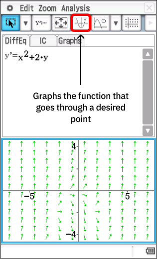
and click on point of the graph we want the function to go through. Alternatively you can click and drag existing points to change where their functions go through.

Conclusion

Hopefully now you have a basic grasp of your Classpad’s capabilities and can see why it outshines your regular scientific calculator. As stated previously, if you’re confused on the use-case of a specific function mentioned in this article, it’s likely that you simply haven’t yet learned the topic relevant to the function, so don’t stress. From here, I recommend you check out the second part to this Classpad guide to really optimise your Classpad efficiency.

Good luck, and happy Classpadding!